Industrial Hygiene Exposure Assessments: Worst-Case vs. Random Sampling

BY JEROME SPEAR, CSP, CIH • J.E. SPEAR CONSULTING, LP

An industrial hygiene exposure assessment is the process used to evaluate a person’s exposure to a chemical or physical agent. However, in order to measure a worker’s “actual” exposure, a monitor would be required to be placed in his/her breathing zone each and every day, which is typically cost prohibitive and time-consuming.

Since it is often impossible (or not practical) to measure every persons’ actual exposures to the chemical or physical agent, judgments regarding the acceptability of exposure are usually made based on an estimate of the person’s dose via representative sampling. However, the exposure assessment strategy that is employed depends on the purpose and goal of the monitoring and what the sample(s) should represent. The two types of sampling strategies to consider when planning an exposure assessment study are “worst-case” sampling and random sampling. The broad difference is that “worst-case” sampling involves more subjectivity than a random sampling approach.

In “worst-case” sampling, workers who are subjectively believed to have the highest exposures are non-randomly selected. If no “worst-case” sample exceeds the occupational exposure limit(s), we can be subjectively satisfied (but not statistically confident) that the exposure profile is acceptable. For example, plant operators who have similar job duties within a production unit of a plant may be identified as a similar exposure group (SEG). For such workers, a “worst-case” exposure might occur on a day that their process unit generates the highest production output. Such a day would subjectively be considered the “worst-case” exposure period and targeted for evaluation.

A random sampling strategy requires workers within a SEG and the sample periods to be randomly selected and subsequent statistical analysis of the exposure data. Decisions on the acceptability of the exposure profile can then be determined with a known level of confidence based on the central tendency and spread (or dispersion) of the sample distribution. Some applications of a random sampling strategy include the following:

Describe the 8-hour time-weighted average (TWA) concentrations over different days for a single worker or SEG.
Describe the 15-minute TWA concentrations over one workshift for a single worker or SEG.
Estimate the full-shift TWA concentration over one workshift based on short-term (or grab) samples for a single worker or SEG.

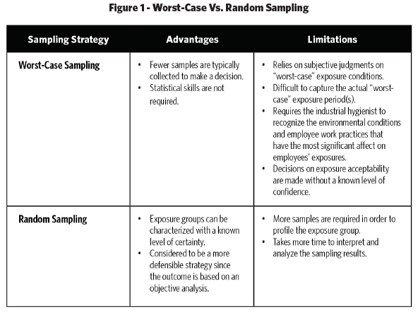
Both “worst-case” sampling strategies and random sampling strategies have their advantages and limitations. The primary advantage of using a “worst-case” sampling strategy is that fewer samples are required to be collected, making it less costly and less time consuming than using a random sampling approach. A limitation with employing a “worst-case” sampling strategy is that it requires the industrial hygienist to recognize the “worst-case” conditions, which may include a “worst-case” exposure judgment about the specific task and/or a specific work practices unique to an individual worker.

However, because our judgment is usually not as good as we think, “worst-case” (i.e., judgmental samples) are likely to contain our own built-in biases. As a result, there is no way to measure the accuracy of “worst-case” samples (Albright, Winston, & Zappe, 1999) and the conclusions about exposure include potential biases of our judgments on the conditions of the job, work practices, and/or other conditions that we believe have an impact on exposure. On the other hand, random sampling
of exposures eliminates such biases since samples of the population are selected via a random mechanism. As a result, the variability in the data (due to work practice variations between workers, day-to-day variations, process variations, etc.) is measured and used to estimate the exposure parameters. Thus, a random sampling strategy is based on an objective analysis of the SEG. Figure 1 provides a comparison of a “worst-case” sampling strategy versus a random sampling strategy .

Statistically speaking, there’s always a chance of making the wrong decision no matter how confident we are but by quantifying our level of certainty through a random sampling strategy, we are able to maximize our chance of making the right decision.

With the availability of computers and statistical software programs available today, much of the statistical “grunt” work can be performed for us making it easier to employ a random sampling strategy. However, there are some statistical terms and considerations that should be understood, which are briefly described in the following 8-step process to exposure profiling.

1. 1. - 1. Identify the SEG to profile. The key point in categorizing SEGs is to select the exposure group in order to minimize the amount of variation between the samples; otherwise, the resulting confidence intervals (calculated from the mean and variance) will be too wide to be useful. A SEG may be a single worker performing a single task; however, it is often impractical to perform random sampling for each and every worker. So, a more practical approach is to include multiple employees in a SEG who have similar exposures. For example, employees assigned to operate propane-powered lift trucks in a warehouse may be grouped as having similar potential exposures to carbon monoxide. If there are multiple SEGs identified (as most facilities have), a method to prioritize the data collection needs can be devised. AIHA’s A Strategy for Assessing and Managing Occupational Exposures, 3rd (2006) provides a method for prioritizing SEGs for study based on the toxicity of the material, conditions of the workplace environment and their likelihood to influence exposures, and individual work practices that are likely to influence exposures.
      2. Randomly select workers and exposure periods within the SEG selected for study. A random sample is one where each worker and time period has an equal probability of being selected for sample collection. It’s important to collect the samples as randomly as possible; otherwise, the resulting statistics will be biased. A random number table and/or the random number function in a spreadsheet computer program (such as Microsoft Excel) are useful tools in the random selection process. Another consideration is, “how many samples should be collected in order for the exposure profile to be useful?” The answer depends on a number of factors, including the variability of the sample. However, AIHA generally recommends between six and 10 samples are needed in order to perform a baseline exposure profile (AIHA, 2006).
      3. Collect breathing zone samples of the randomly selected workers at randomly selected time periods. Breathing zone samples should be collected near the employee’s nose and mouth. The breathing zone can be visualized as a hemisphere about six to nine inches around the employee’s face. Personnel conducting industrial hygiene exposure monitoring should have at least an understanding of the nature of the job or process in which the agent(s) is used or generated and also have a basic understanding in field sampling methods and techniques. Although some formal training and/or hands-on training on exposure monitoring techniques and analytical methods are useful, the mechanics of conducting personal air sampling can be self-taught. There are several sources of information that are helpful in identifying the appropriate sampling and analytical methodology and equipment. Such resources include OSHA’s Technical Manual and NIOSH’s Manual of Analytical Methods. Also, an AIHA-accredited laboratory can provide guidance and instructions on specific sampling methods.
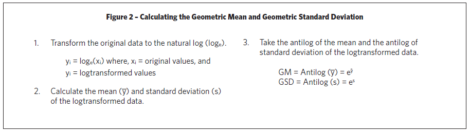
      4. Calculate the descriptive statistics for the data set. Descriptive statistics include the mean, median, percent above the occupational exposure limit (OEL), range, and standard deviation that characterize the sample’s distribution such as the central tendency and the variability in the data. The mean and median are used to measure the central tendency of the data, whereas, the range and standard deviation are measures of variability. By looking at the data from a number of points of view, information and patterns in the data may be discovered. Many data sets can be interpreted simply by comparing the OEL with descriptive statistics. When most of the data are clustered well below or well above the OEL, a decision can generally be made on workplace acceptability by using descriptive statistics (AIHA, 2006). The geometric mean (GM) and geometric standard deviation (GSD) are descriptive statistics that are used to estimate parameters of a lognormal distribution (see Step 5 below). The GM is the antilog of the arithmetic mean of the log-transformed values (see Figure 2). The GM is the value below and above which lie 50% of the elements in the population (i.e., the population median). The GSD is the antilog of the standard deviation of the log-transformed values (see Figure 2). The GSD is unitless and reflects variability in the population around the GM; therefore, confidence intervals will have a larger spread as the GSD increases.
      5. Determine if the data fits a lognormal and/or normal distribution. 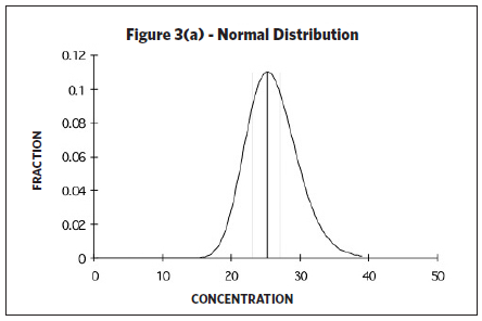Upper and lower confidence limits and upper tolerance limits are calculated based on knowing (or assuming) a certain underlying distribution of the data set. The type of distribution (i.e., normal or lognormal) will generate different confidence intervals and tolerance limits. A random variable is called normally distributed if the distribution (as plotted on a histogram) looks like a bell-shaped curve. However, industrial hygiene sampling data is often “skewed to the right” (see Figure 3(b)) since occupational exposure values have a lower boundary (i.e., the measured exposure value cannot be less than zero). Taking the log of the variable often mitigates such skewness. In such cases, the distribution is then considered lognormally distributed, or lognormal, if the log of the 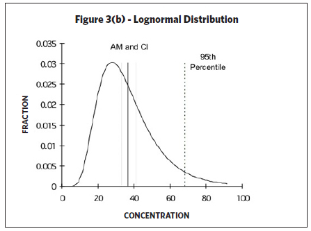variable is normally distributed. The lognormal distribution is often applied to occupational exposures, yet the assumption of lognormality is seldom verified (Waters, Selvin, & Rappaport, 1991). If the data follows neither a lognormal nor a normal distribution, the data may not represent a single SEG. In such cases, the data may need to be divided into two or more SEGs and analyzed separately (AIHA, 2006). If the sample size is large with lots of values, the data can be visualized by creating a histogram of the data (i.e., plotting the relative frequency of elements falling in specified intervals). However, industrial hygiene sampling data sets often consists of small data sets with fewer than 10 samples due to cost and/or other constraints. One way to qualitatively determine if the underlying distribution follows a lognormal and/or normal distribution for small sample sizes is to plot the data on probability paper. A lognormal distribution is suggested if the data plotted on lognormal probability paper forms a straight line. Likewise, a normal distribution is suggested if the data plotted on normal probability paper forms a straight line. A major advantage of probability plotting is the amount of information that can be displayed in a compact form but it requires subjectivity in the deciding how well the model fits the data (Waters, Selvin, & Rappaport, 1991) since probability plotting relies on whether or not the plotted data forms a straight line. Identifying large deviations from linearity is based on the subjective valuation of viewing the probability plot. Probability paper is available for various types of sample distributions and plotting procedures are described in Technical Appendix I of the NIOSH Occupational Exposure
        Sampling Strategy Manual (Leidel, Busch, & Lynch, 1977). If a statistical program is available, a more quantitative approach should be used to evaluate the goodness-of-fit of the distribution. If both a lognormal and normal distribution is indicated, the confidence limits and upper tolerance limit should be calculated assuming a lognormal distribution.
      6. Calculate the estimated arithmetic mean, one-side upper and lower confidence limits of the arithmetic mean, 95th percentile, and the upper tolerance limit for the data set.
        
        Estimated arithmetic mean – For a normal distribution, the estimated arithmetic mean is the same as the sample mean. However, if the data is lognormally distributed, there are several methods for estimating the arithmetic mean and for calculating confidence limits. The sample mean and t-Distribution confidence limits (see Figure 4) have the advantage of being easy to calculate but can be more variable than other estimates (AIHA, 2006). Other preferred methods for estimating the arithmetic mean and computing the confidence limits are described in AIHA’s A Strategy for Assessing and Managing Occupational Exposures, 3rd Edition (2006) but estimating the arithmetic mean and computing the confidence limits using such preferred methods are difficult to compute without the use of a computer and/or specialized software.
        
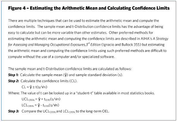
        UCL1,95% and LCL1,95% of the arithmetic mean – For evaluating toxicants that produce chronic diseases, the mean exposure should be examined (Rappaport & Selvin, 1987). However, to evaluate acute (short-term) exposures, the upper tolerance limit of the 95th percentile should be examined. The UCL1,95% is the one-sided upper value at a 95% confidence level. Likewise, the LCL1,95% is the one-sided lower value at a 95% confidence level. If the UCL1,95% is below the OEL, there is a 95% confidence level that the long-term average exposure is below the OEL. However, from an OSHA compliance officer’s perspective, the burden of proof is on the compliance officer to show that the worker was overexposed with at least 95% certainty. Therefore, the OSHA compliance officer must demonstrate that the LCL1,95% exceeds OSHA’s permissible exposure limit (PEL). If the data is lognormally distributed, there are different methods to calculating the confidence limits for the arithmetic mean. The sample mean and t-Distribution confidence limits (see Figure 4) have the advantage of being easy to calculate but can be more variable than other estimates (AIHA, 2006) as previously discussed.
        
        95th percentile – The 95th percentile is the value in which 95% of the population will be included. For example, the median is the 50th percentile.
        
        UTL95%,95% – The UTL95%,95% is the upper tolerance limit of the 95th percentile and is typically used to examine acute (or short-term) exposures (i.e., fast-acting contaminants). For a lognormal distribution, the UTL95%,95% is calculated by the following: UTL95%,95% = e (ȳ + K s) (AIHA, 2006) where, ȳ and s are the mean and standard deviation, respectively, of the log-transformed data. “K” is a factor for tolerance limits that is obtained from a table given the confidence level, percentile, and number of samples.
      7. Make a decision on the acceptability of the exposure profile. Generally, an UCL1,95% that results in a value greater than the long-term OEL suggests that the exposure profile is unacceptable; whereas, an UCL1,95% that results in a value below the long-term OEL suggests that the exposure profile is acceptable. For chemicals with acute (or short-term) effects, the upper tolerance limit of the 95th percentile should be examined. However, calculating the UTL95%,95% with few data points tends to produce a wide tolerance interval, which limits its usefulness. An UTL95%,95% that results in a value below the short-term exposure level and ceiling limit suggests that the exposure profile is acceptable, but large numbers of samples are needed in order to identify “acceptable” environments (Selvin, Rappaport, Spear, Schulman, & Francis, 1987).
      8. Refine the SEG, if necessary. The results of the exposure profile may indicate that the exposure group may need to be further refined. For example, it may appear that the sampling for certain individuals seem to result in higher exposures. To statistically test the significance of this variation, an analysis of variance (ANOVA) may be performed. An ANOVA is an inferential statistical test that compares two or more means to determine if the means are significantly different. If the means are statistically different, the SEG may need to be further refined.

To illustrate a random sampling approach, two case studies are described below. One describes how to evaluate the exposure of a single worker using a random sampling method. The other involves estimating a full-shift TWA based on random short-term samples.

Example 1: Estimating the Long-Term Exposure of a Single Employee

An employer requested to evaluate a particular employee’s 8-hour TWA exposure (in relation to OSHA’s PEL) to formaldehyde during a manufacturing task. The first step in assessing exposures to environmental agents is to have a thorough understanding of the processes, tasks, and contaminants to be studied. Information may be obtained through observations and possibly the use
of direct-reading devices. Interviews with workers, managers, maintenance personnel and other relevant personnel (such as technical experts) provide an additional source of information and knowledge. In addition, a review of records and documents (including past exposure monitoring data), relevant industry standards, and/or other literature can provide some insights on the magnitude of exposures for given processes and tasks performed at the work site. In this case, the employee operates equipment that forms fiberglass-matting material that is used in building materials (such as backing for shingles). Potential of formaldehyde exposure was identified since formaldehyde was listed as a component in the resin used to bind the fiberglass matting based on a review of the material safety data sheet.

To assess this employee’s exposure using a “worst-case” sampling strategy, breathing zone air samples would be collected on days believed to exhibit the highest exposure to formaldehyde. The sampling results would then be used to derive conclusions based on our judgments (and potential biases) of “worst-case” conditions. However, to eliminate potential biases or incorrect “worst-case” exposure judgments, a random sampling strategy was designed.

A total of five workdays were randomly selected, which represented the 8-hour sample periods. A formaldehyde monitor was then placed in the employee’s breathing zone for the duration of the randomly-selected workdays to measure the TWA concentration of formaldehyde. The descriptive statistics were calculated, which resulted in the following:

Maximum: 0.85 ppm
Minimum: 0.43 ppm
Range: 0.42 ppm
Mean: 0.624 ppm
Median: 0.60 ppm
Standard deviation: 0.15 ppm
Geometric mean: 0.610 ppm
Geometric standard deviation: 1.274 ppm

The above descriptive statistics indicates no substantial outliers in the data since the mean and median are relatively close in value.
Next, to ensure that the data follows a normal and/or lognormal distribution, the data was plotted on probability paper and a statistical goodness-of-fit test was performed, which indicated both a lognormal and normal distribution. As a result, the arithmetic mean, UCL1,95%, and UCL1,95% were estimated assuming a lognormal distribution, which are provided below:

Estimated arithmetic mean: 0.624 ppm
UCL1,95%: 0.823 ppm
LCL1,95%: 0.512 ppm

In this example, we can conclude that, with 95% certainty, this employee’s exposure to formaldehyde will be less than 0.823 ppm on any given workday. Although the mean concentration of formaldehyde (i.e., 0.624 ppm) for this employee is less than OSHA’s PEL of 0.75 ppm, the most conservative approach would be to reduce exposures to a level less than the UCL1,95%. Therefore, from the employer’s perspective who is concerned with ensuring a safe workplace, additional interventions to reduce this employee’s formaldehyde exposure are warranted since the employer cannot conclude, with 95% certainty, that his exposure is below the PEL. However, from an OSHA compliance officer’s perspective, the burden of proof is on the compliance officer to show that the worker was overexposed, with at least 95% certainty. In this case, the compliance officer would be unable to demonstrate that that the employee’s exposure exceeds the PEL, with 95% certainty, since the LCL1,95% is less than the PEL.

Example 2: Estimating the TWA Concentration Based on Random Short-Term Samples

A potential exposure of 1,6-hexamethylene diisocyanate (HDI) to painters during the spray painting of an exterior shell of an above ground storage tank was identified by the employer. Due to limitations with the selected field sampling and analytical method for HDI, the sample duration was required to be limited to approximately 15 minutes. The spray-painting task was performed by painters working from a boom-supported elevated platform. At times, two painters worked from the same platform and at other times, only one painter performed the task. As a result, a sampling strategy was developed that involved the use of both a “worst-case” and a random sampling approach. Due to the sampling duration limitations, that sampling strategy included collecting random, short-term samples from the breathing zone of each painter and to estimate the TWA concentration for the task based on the short-term samples. However, the “worst-case” exposure condition was also targeted. That is, random short-term samples were collected when both painters worked side-by-side from the same elevated platform since this condition was assumed to represent the highest exposures to the painters.

Four random, short-term samples were collected from the breathing zone of each painter (i.e., a total of eight random samples), which resulted in the following descriptive statistics:

Maximum: 0.0042 mg/m3
Minimum: <0.00037 mg/m3
Range: 0.00394 mg/m3
Mean: 0.002 mg/m3
Median: 0.002 mg/m3
Standard deviation: 0.001 mg/m3
Geometric mean: 0.002 mg/m3
Geometric standard deviation: 2.545 mg/m3

The descriptive statistics above indicate no significant outliers in the data since the mean and median are equivalent.

To ensure that the data follows a normal and/or lognormal distribution, the data was plotted on probability paper and a statistical goodness-of-fit test was performed, which indicated both a lognormal and normal distribution. As a result, the arithmetic mean, LCL1,95%, and UCL1,95% were estimated assuming a lognormal distribution, which are provided below:

Estimated arithmetic mean: 0.002 mg/m3
UCL1,95%: 0.007 mg/m3
LCL1,95%: 0.001 mg/m3

In this example, we can conclude, with 95% certainty, that the TWA concentration of HDI for the task is less than 0.007 mg/m3. Since the UCL1,95% is below the PEL of 0.034 mg/m3, the exposure was determined to be acceptable from both the employer’s perspective and the OSHA compliance officer’s perspective.

It is important to note that this case study does not account for day-to-day variation that may exist since the sampling was limited to periods within a single workshift. Therefore, the results represent the TWA concentration for the task that was performed on the date of the sampling. However, this TWA concentration represents the “worst-case” condition for this task since breathing zone samples were collected during “worst-case” conditions (i.e., when two painters were spray painting from the same platform).

Historically, more attention has been given to airborne exposures than exposures to physical agents and dermal exposures. However, there are many situations in which random sampling strategies may be applied to data other than airborne samples. For some chemicals, skin absorption may be the predominant route of exposure and airborne samples would not be the most appropriate variable to study such exposures. Biological monitoring may be more appropriate to study for such circumstances.

Random sampling approaches may also be applied to physical agents. However, for noise data and/or other variables measured in a logarithmic scale, analyzing the allowable dose (i.e., percent of dose), rather than decibels, should be considered so that statistical tools can be applied to such exposure measurements.

In summary, both worst-case sampling and random sampling strategies are useful in assessing exposures. It is important to understand the limitations of each and to correctly apply the chosen sampling strategy. A primary benefit of a random sampling strategy is that it allows SEGs to be profiled with a known level of certainty, which makes it a more defensible and objective sampling strategy. Conversely, the primary benefit of a “worst-case” sampling approach is that fewer samples are needed (thereby less costly and less time consuming) to make an exposure judgment. In some cases, both a combination of a “worst-case” and a random sampling strategy may be beneficial.

Print Friendly